One-Sample T-Test in SPSS
A one-sample t-test is a statistical method used to determine whether the mean of a single sample significantly differs from a known or hypothesized population mean. This test is particularly useful when researchers or analysts have a specific target or reference value and want to assess how a sample's mean compares to that value. By evaluating the sample mean against the population mean, the one-sample t-test helps identify whether observed differences are likely due to random chance or if they indicate a statistically significant deviation.
Introduction to One-Sample T-test
Commonly used in fields such as psychology, education, and medical research, the one-sample t-test provides a straightforward way to test hypotheses about population means, especially when dealing with small sample sizes and when the population standard deviation is unknown.
In certain studies, researchers aim to compare the mean score from a single sample to a standard or reference value. For instance, a health researcher might be interested in determining if the average blood pressure of a population has changed compared to the average blood pressure from several decades ago. The average blood pressure from that time serves as the reference value. The researcher randomly selects a sample from the current population, records their average blood pressure (and standard deviation), and seeks to determine if there has been an increase or decrease compared to the past population's average blood pressure. The researcher does not have access to individual data from decades ago, only to the reference. However, individual data from the current population is available, allowing the calculation of both the mean and standard deviation. To assess whether the current average blood pressure significantly differs from the historical average, the researcher performs a one-sample t-test.
An important assumption when conducting a one-sample t-test is that the data should be normally distributed and the observations must be unrelated to each other.
In the following sections, we present an example research scenario where a one-sample t-test will be used to analyze the data. We will demonstrate how to perform a one-sample t-test in the SPSS program step-by-step and how to interpret the SPSS results output for the one-sample t-test.
One-Sample T-test Example
Is the average arsenic level in the school drinking water pipes within the limits of the EPA standard?

A high school science class aimed to determine if the drinking water quality in high schools within neighboring urban areas meets the Environmental Protection Agency (EPA) safety standards. Drinking water quality is assessed by measuring various organic and chemical compounds, including arsenic. According to the EPA, the acceptable level of arsenic in drinking water is 10 μg/L. The students randomly selected 32 high schools and collected water samples from the school building pipes on a school day. They then analyzed the water samples in their school laboratory to measure the arsenic levels. Table 1 displays the amount of arsenic found in the water from five schools.
| School | Arsenic Level in Water(μg/L) |
|---|---|
| School01 | 6.29 |
| School02 | 7.64 |
| School03 | 5.98 |
| School04 | 6.92 |
| School05 | 8.09 |
| ... | ... |
The science class is interested in determining whether the mean arsenic level in the sampled water meets the EPA standard. If the sample mean is less than or equal to the standard, it is considered safe. If it is slightly higher, it may still be acceptable. However, if it is statistically significantly higher, it raises concern.
The teacher enters the data in the SPSS program in the hospital computer lab. The data for this example can be downloaded in the SPSS format or in CSV format.
Entering Data into SPSS
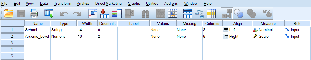
To enter the data in the SPSS program, first we click on the Variable View tab (bottom left) and create two variables under name column: School, Arsenic_Level. We specify the following attributes for each variable:
- School: Data type is String. Measurement level is Nominal
- Arsenic_Level: Data type is Numeric. Measurement level is Scale
When defining the variables, we must specify both the data type and the measurement level for SPSS. The data type is used by the computer to read the data, while the measurement level is used by the statistical algorithm for computation. In this example, the School variable consists of names and is not involved in the computation, so we select "string" as the data type and "nominal" as the measurement level. Figure 1 shows how the variable specification should look like in the SPSS Variable View for this example.
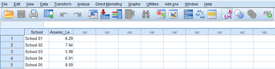
After creating the variables in the Variable View tab, we navigate to Data View and enter the data. We can either enter the data directly into the cells by hand or copy and paste from a spreadsheet. Figure 2 shows the blood pressure data for the first five participants in the Data View window of the SPSS program.
Now we are ready to conduct a one-sample t-test in SPSS!
Analysis: One-sample T-test in SPSS
A one-sample t-test is a statistical method used to compare the mean score of a single random sample to a known or hypothesized population mean or a reference value. In our study scenario, the science class aims to determine if the arsenic levels in drinking water from high schools in neighboring urban areas meet the standard set by the Environmental Protection Agency (EPA). The acceptable arsenic level according to the EPA is 10 μg/L. The students measure the arsenic levels in water samples from 32 high schools and compare the sample mean to the EPA standard using the one-sample t-test. This test helps assess whether the observed mean arsenic level in the sampled water is significantly different from the reference value set by the EPA.
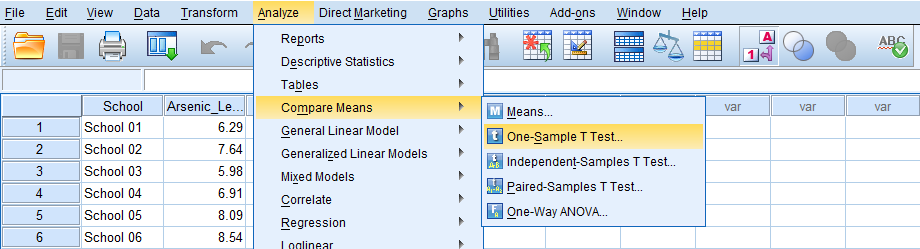
In SPSS, the one-sample t-test can be accessed through the menu Analyze/Compare Means/One-Sample T Test. As shown in Figure 3, we click on Analyze, then choose Compare Means, and finally select One-Sample T Test.
By clicking on One-Sample T Test, a window will appear that asks for the test variable (Arsenic level) and the test value (the standard or reference we are comparing with). The test variable is the variable whose mean we want to compare with. The test value is the reference value we want to compare our test (sample) variable mean against. Because we are investigating if the average arsenic level is different from the EPA standard of 10 (μg/L) or less, we enter the reference value of 10 in the test value box, as shown in Figure 4 below.
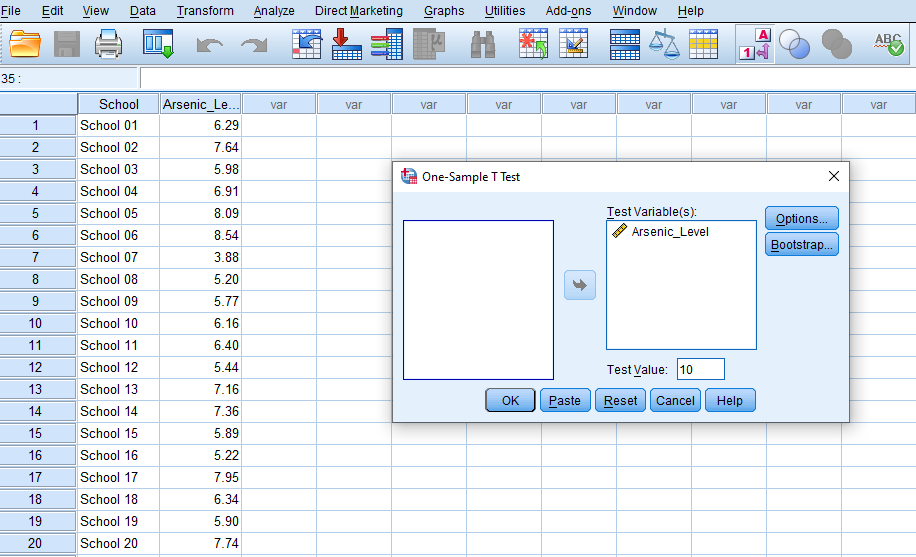
Once we press the OK button to run the one-sample t-test, SPSS will produce the results of one-sample t-test.
Interpretation: One-Sample T-test in SPSS
In this study, the science class aimed to determine if the arsenic levels in drinking water from high schools in neighboring urban areas met the Environmental Protection Agency (EPA) standard. A one-sample t-test was conducted to compare the mean arsenic levels in the sampled water to the EPA's acceptable level of 10 μg/L. The SPSS results for the one-sample t-test include two tables: a table for descriptive statistics (One-Sample Statistics), and a table for the One-Sample Test results (One-Sample Test).
Figure 5 displays the One-Sample Statistics table, which includes the sample size (N = 32), the mean arsenic level in drinking water (Mean = 6.379), the standard deviation from the mean (1.283), and the standard error of the mean (0.227).
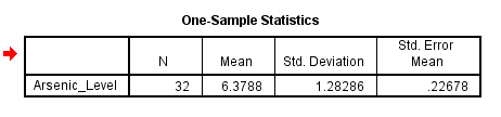
According to the descriptive statistics, the mean value for the arsenic level is 6.379 (μg/L), which is below the maximum threshold of 10 (μg/L), which is good news. But is a mean value of 6.379 (μg/L) statistically significant below the reference set by EPA? We can determine this by referring to the One-Sample Test table (the second table in the SPSS output and Figure 6 below).
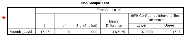
As Figure 6 above shows displays, the Mean Difference is -3.621 (i.e., the difference between the sampled water mean arsenic level and the standard set by EPA), which is statistically significant with t=-15.968, df=31, and p=0.000. In addition, the null hypothesis value of zero difference is not inside the 95% confidence intervals [-4.083, -3.158], further ensuring that the null hypothesis can be rejected.
Reporting the Results of One-Sample T-test
In this study, the science class aimed to assess whether the arsenic levels in drinking water from high schools in neighboring urban areas met the Environmental Protection Agency (EPA) standard. The EPA has set the acceptable level of arsenic in drinking water at 10 μg/L. To evaluate the water quality, the students randomly selected 32 high schools and measured the arsenic levels in water samples collected from the school building pipes on a school day.
A one-sample t-test was conducted to compare the mean arsenic level in the sampled water to the EPA standard. As displayed in Figure 6, the mean difference between the sampled water arsenic level and the EPA standard was -3.621. This difference is statistically significant, with a t value of -15.968, degrees of freedom (df) of 31, and a p value of 0.000 (p < 0.01). The null hypothesis value of zero difference is not within the 95% confidence intervals [-4.083, -3.158], further confirming that the null hypothesis can be rejected.
The results indicate that the mean arsenic level in the drinking water samples from the selected high schools is significantly lower than the EPA standard of 10 μg/L. This finding suggests that the drinking water quality in these high schools is within the safe limit set by the EPA for arsenic levels. However, continuous monitoring and testing are recommended to ensure the water quality remains safe for consumption.