One-Way ANOVA in SPSS
The one-way analysis of variance or one-way ANOVA is a statistical method that compares the mean values of several groups on a continuous dependent variable to determine if any difference in mean values across the groups is statistically significant. One-way ANOVA is usually used when the number of groups for comparison is three or more. However, one-way ANOVA can also be used instead of independent samples t-test to compare the mean values between two groups. A one-way ANOVA is usually followed by a pairwise group comparison tests, technically called post hoc tests.
Introduction to One-Way Analysis of Variance
There are situations where researchers are interested in comparing the mean values across three or more groups. For example, a researcher may be interested in investigating the effect of different education levels (high school and lower, bachelor's degree, graduate degree) on income. In this example, education level has three levels / groups and is the independent variable or the factor and income is the dependent variable, which is continuous.
When using ANOVA, the independent variable is also called a factor. A factor is a categorical variable with two or more categories or levels. For example, education attainment is a factor with three levels: high school and lower, bachelor’s degree, and graduate degree. Because the independent variable is called a factor in ANOVA analysis, experimental designs using ANOVA may be referred to as factorial designs. If the research design has only one factor, we call the analysis of variance as one-way ANOVA, which is the traditional name for one-factor ANOVA. If the research design includes two factors, it is called a two-way ANOVA, and so on. The term factorial ANOVA is sometimes used to denote two-way or more factors in the design.
In an ANOVA test, the primary purpose is to see if the factor as the aggregate of its categories has a significant effect on the dependent variable. If the effect of factor on the dependent variable is statistically significant, then we want to know which categories are significantly different from each other. If the factor overall is not statistically significant, we stop there and do not compare its constituent categories.
In the following sections, we present an example research scenario where a one-way ANOVA will be used to analyze the data. We will demonstrate how to perform a one-way ANOVA in SPSS step-by-step and how to interpret the SPSS results output.
One-way ANOVA Example
Does the type of physical therapy affect the recovery time of patients after knee surgery?
A health researcher conducts a study to investigate whether different types of physical therapy affect the recovery time of patients after undergoing knee surgery. The study includes three groups of patients:
- Group 1: Patients receiving no physical therapy (Control)
- Group 2: Patients receiving Standard physical therapy
- Group 3: Patients receiving Advanced physical therapy
After the surgery, the researcher records the number of days it takes for each patient to fully recover. Patients have been randomly recruited from different sites and randomly assigned to each physical therapy group. Recovery time is recorded when the physical therapist certifies full recovery, and the patient feels comfortable in walking. Recovery time is recorded in days.
In this study design, there is one factor (Physical therapy method) with three categories / groups (Standard physical therapy, Advanced physical therapy, No physical therapy or the Control) and the measure (recovery time) is continuous, therefore, a one-way ANOVA would be appropriate to address the research question. If the ANOVA results are significant, post hoc tests can be conducted to identify which specific groups differ from each other. Table 1 shows the recovery time in days of six knee injury patients in three different physical therapy treatments.
| Patient | Group | Recovery Time |
|---|---|---|
| P1 | Control | 34 |
| P10 | Control | 36 |
| P26 | Standard | 24 |
| P36 | Standard | 23 |
| P50 | Asvanced | 28 |
| P60 | Advanced | 17 |
| ... | ... | ... |
The researcher is interested in knowing if the physical therapy method has an effect on the recovery time of the knee injury patients and if positive, which therapy method is more effective than the others. The researcher enters the data in the SPSS program in the hospital computer lab. The data for this example can be downloaded in the SPSS format or in CSV format.
Entering Data into SPSS
To enter the data in the SPSS program, first we click on the Variable View tab (bottom left) and create three variables under name: Patient, Method, Recovery_Time. We specify the following attributes for each variable:
- Patient: Data type is String. Measurement level is Nominal
- Method: Data type is Numeric (Values are 1: Control, 2: Standard, 3: Advanced), Measurement level is Nominal
- Recovery_Time: Data type is Numeric, Measurement level is Scale
When defining the variables, we must specify both the data type and the measurement level for SPSS. The data type is used by the program to read the data, while the measurement level is used by the statistical algorithm for computation.
In this example, the Patient variable consists of patient ID’s and is not involved in the computation, so we select "string" as the data type and "nominal" as the measurement level.
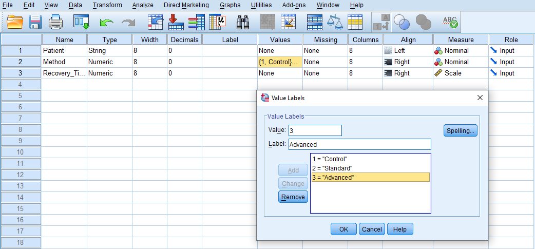
For the Method variable, although they are names of physical therapy methods (Control, Standard, Advanced), we assign numbers to them. So, we choose "Numeric" as the data type but select "Nominal" as the measurement level. To assign numbers with the types of physical therapy methods, in the Value column, click on the cell in the Method row to open a window. In the Value box, enter 1 and in the Label box, enter "Control," then click "add." Repeat this process with Value 2 for the "Standard" and value 3 for “Advanced” and close the window. Figure 1 shows how to create Method levels (Control, Standard, Advanced) and assign numbers to them.
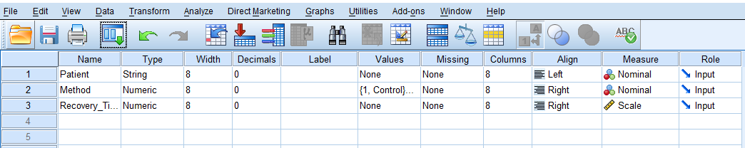
The data type for the variable Recovery_Time is also "Numeric," and for the measurement level, we select "Scale." After creating all variables, the Variable View panel of SPSS for our dataset should look like Figure 2.
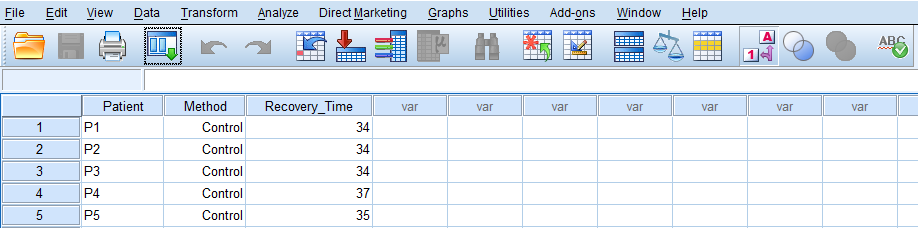
Once the variables are created, we can enter the data into the columns Patient, Method, and Recovery_Time in the Data View tab of SPSS program. For Patient, we can enter their names or an ID. For the variable Method, we can either directly type the method name (Control, Standard, Advanced), or the values we assigned them during the variable creation step in the Variable View tab (1, 2, 3). In the latter case, we can enter 1 for “Control”, 2 for the “Standard”, and 3 for “Advanced”. Finally, we enter the days of recovery time in the Recovery_Time column. Figure 3 shows how the data for all three variables should look like in the Data View tab.
Now we are ready to conduct the one-way ANOVA in SPSS
Analysis: One-way ANOVA in SPSS
A one-way ANOVA is a statistical method for comparing the means between two, three or more groups. In our study scenario, the health researcher is interested in knowing if different physical therapy methods (Control, Standard, Advanced) have significant effect on the recovery time (in days) of knee injury patients after their surgery. In addition to the Standard and Advanced groups, the researcher assigns some patients to the Control group. So, there are three groups overall: Control, Standard, Advanced. For three groups or levels of a factor, we can use the one-way ANOVA to compare their means on Recovery time.
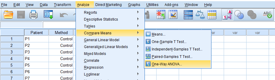
In SPSS, the one-way ANOVA test can be accessed from the menu Analyze / Compare Means / One-Way ANOVA. So, as Figure 4 demonstrates, we click on Analyze and then choose Compare Means and then One-Way ANOVA.
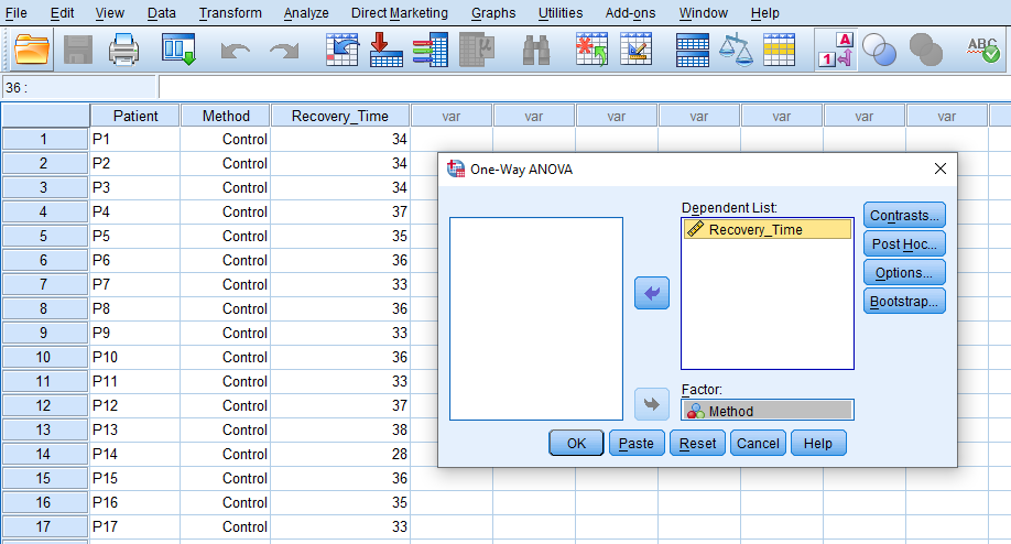
After clicking on One-Way ANOVA, a window will appear asking for Dependent List (i.e., dependent variables) and the Factor (i.e., independent variables). We send Recovery_Time into the Dependent List box and the Method into the Factor box. Figure 5 shows how the window should be populated with our dependent and independent variables.
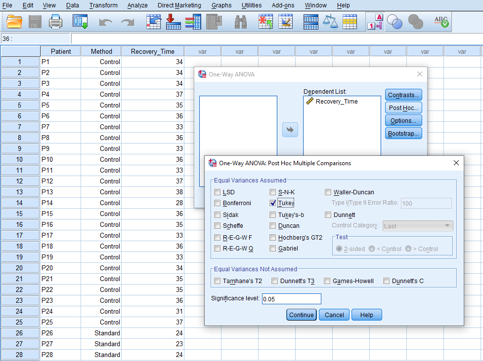
In addition to performing a one-way ANOVA, we are also interested in knowing which physical therapy method produces better results (i.e., shorter recovery time). In other words, we would like to compare Standard method against the Control, Advanced method against the Control, and Advanced method against the Standard method. These pair-wise tests are called post hoc tests because they are performed after the one-way ANOVA general (omnibus) test. So, in the open window, we click on Post Hoc and choose the Tukey test (Figure 6).
After choosing the Tukey test as our post hoc test, we close this window by clicking on Continue.
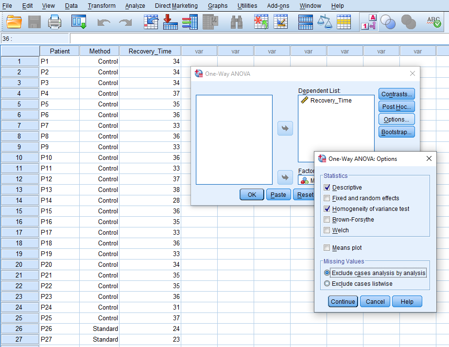
Because we want to know which mean value is significantly different from others, we also need to obtain some descriptive statistics. So, we click on Options and select Descriptive and Homogeneity of Variance Test. The Homogeneity of Variance Test performs Levene's test for homogeneity of variance to test the assumption that the variances of the three groups on the dependent variable are equal. This assumption is especially required if the group sizes are different. Figure 7 shows the window to choose these two options from.
We then click on Continue and then on OK buttons to run the one-way ANOVA test.
Interpretation: One-way ANOVA in SPSS
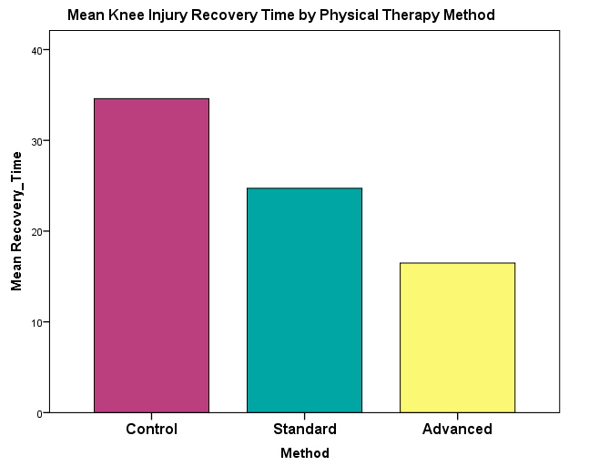
In this study, the researcher is interested in investigating the effectiveness of the Standard and Advanced physical therapy method on knee injury patients’ recovery time (in days). In addition to the two Standard and Advanced physical therapy methods, there is a third group that includes the control patients (patients receiving no physical therapy voluntarily). The researcher performs a one-way ANOVA to compare the mean recovery times across the three groups. The mean recovery time for different physical therapy methods is shown in Figure 8 below.
The results of the SPSS one-way ANOVA include a table for descriptive statistics (Descriptives), a table for the results of the homogeneity of variance test (Test of Homogeneity of Variance), the ANOVA table, the table of post hoc tests (Multiple Comparison) and a table showing the Homogenous Subsets. We will go through each of these tables in the output.
The first table in the output is the descriptive statistics table (Figure 9), which includes the mean, standard deviation, the standard error, the confidence intervals of the means, and the minimum and maximum values.
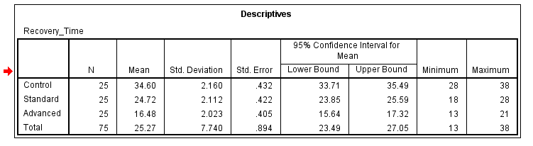
In the Descriptives table, we can see that the mean recovery times for the Control, Standard, and the Advanced groups are 34.60 days, 24.72 days, and 16.48 days, respectively. We guess that differences between the average scores are noticeable. In particular, the shortest recovery time happens in the Advanced physical therapy method.
The second table in the output shows the results of the homogeneity of variance test. In ANOVA, we assume that the variances of the dependent variable values in different groups are equal or homogenous, especially when the sample sizes are unequal. Otherwise, the results could be unreliable. The Levenes’ test of homogeneity of variances shows if the variances across the groups are equal (not statistically significantly different from each other). Figure 10 shows the results of the homogeneity test of variance in our example data set.
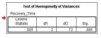
According to the table in Figure 9, the variances across the three groups are not significantly different from each other (p >> 0.05), and we conclude that the assumption of homogeneity of variance is satisfied.
The next table shows the ANOVA test results (Figure 10 below). The ANOVA test (also called the omnibus ANOVA) shows the overall effect of the physical therapy method (regardless of the individual methods). If the overall ANOVA test shows statistically significant results, then we can go further and look at pairwise comparisons. Figure 11 shows the ANOVA table.
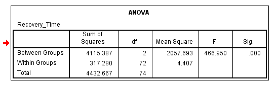
In the ANOVA table in Figure 11, the Between Groups row shows that with an F = 466.950 and degrees of freedom 2 and 72, the model overall is significant with p < 0.05. Therefore, we conclude that the physical therapy method overall has a statistically significant effect on the recovery time of knee injury patients.
Now, we may ask which physical therapy method is better, the Standard or the Advanced? Of course, the descriptive statistics table showed us an apparent answer. But is the difference between the methods statistically significant? We can look at the post hoc test results in the Multiple Comparison table to address this question. The multiple comparison table is shown in Figure 12.
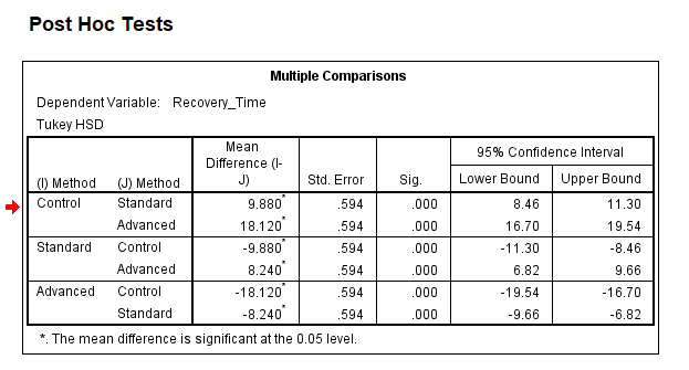
According to the Multiple Comparison table above, there are three pairwise comparisons: between Control and Standard (difference in means = 9.880), between Control and Advanced (difference in means = 18.120), and between Standard and Advanced (difference in means = 8.240). The other comparisons are just repeats of these, with order reversed. According to the Sig. column, all mean differences are statistically significant. It implies that patients in Advanced physical therapy treatment method had statistically and significantly shorter recovery time than patients in the Standard treatment method and the Control group. In addition, patients in the Standard treatment group had a statistically significantly shorter recovery time than the Control group, but not shorter than the Advanced group.
The last table in the one-way ANOVA results is the Homogenous Subsets table. A homogenous subsets table creates subsets (columns) and includes in that column the groups which have similar means (not statistically different). The number of subsets (columns) depends on the number of different sets of similar means. For example, if groups 1 and 2 had similar means and both of them were different from group 3, there would be two columns: in column 1 we would have groups 1 and 2 (because they are similar by their means), and in column 2 we would have group 3 because group 3 is different from the set of groups 1 and 2. In our data set, the homogenous table produces three columns each with only one group (shown by numbers 1, 2, 3). Figure 13 shows the homogenous table for physical therapy data.
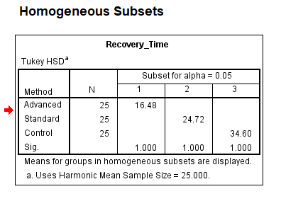
As Figure 11 shows, there are three subsets (1, 2, 3) and each includes only one group (shown by their means.) For example, subset 1 includes the mean value 16.48 which corresponds to the Advanced group (groups names are shown in the first column Method). Subset 2 includes the mean value of 24.72 (Standard group) and subset 3 includes the mean value 34.60 (Control group). The subsets themselves are significantly different from each other (alpha = 0.05 means a p value of < 0.05). But within each subset, the groups are not different from each other. In our case, there is only one group within a subset, which is not statistically different from itself (hence Sig.=1.000). Homogenous subsets tables are not often used in reporting multiple comparisons.
Reporting the Results of One-way ANOVA
In this research, we were interested in evaluating the effectiveness of different physical therapy programs. A random sample of participants was recruited and randomly assigned to one of the three groups: Control (N = 25), Standard physical therapy (N = 25), and Advanced physical therapy (N = 25). Full recovery from the knee injury was measured in days as verified and reported by the physical therapist. The Control group had a mean recovery time (M) of 34.60, with a standard deviation (SD) of 2.160. The Standard physical therapy group had a mean recovery time (M) of 24.72, with a standard deviation (SD) of 2.112. The Advanced physical therapy group had a mean recovery time (M) of 16.48 with a standard deviation (SD) of 2.023.
A one-way ANOVA was conducted to compare mean recovery times among the three groups. The results showed a significant effect of the therapy program on mean recovery times at the p < 0.05 level for the three conditions [F(2, 72)=466.95, p < .05]. Post hoc comparisons using the Tukey HSD test indicated that the mean score for the Control group was significantly different from both the Standard and Advanced groups. Additionally, the Advanced group had a significantly higher mean score compared to the Standard group.
The results suggest that the Advanced physical therapy program is significantly more effective in reducing recovery time compared to both the Control and Standard programs. The Standard physical therapy program is also more effective than no therapy (Control). These findings support the use of enhanced physical therapy interventions to achieve better patient outcomes and provide a basis for clinicians to consider implementing the Advanced physical therapy program in their practice for the appropriate patient population.