Survival Analysis in SPSS: Cox Proportional Hazard Regression
Cox proportional hazard (PH) regression is a survival analysis regression model that explains the relationship between the survival event incidence and a set of predictors. Cox regression is one of the most common semi-parametric modeling methods in survival analysis in medical and health research. Whereas the Kaplan-Meier curve and the log-rank tests provide insight into difference in survival probability between groups, the Cox regression can provide a multivariate insight into impact of different factors on the event incidence.

Introduction to Cox Proportional Hazards Regression
In survival analysis, we are interested in modeling the time to an event of interest (e.g., death, recovery, relapse, etc.). In addition, we may be interested in knowing how different factors (e.g., age, sex, treatment type) influence the likelihood of the event occurring. Cox proportional hazards regression is a popular method for analyzing survival data and can help us understand the impact of these factors on survival.
Cox regression is a semi-parametric model that does not assume a specific distribution for survival times, making it flexible and widely applicable. The model estimates the hazard ratio (HR) for each predictor, which indicates the relative risk of the event occurring at any given time point, given the presence of that predictor. A hazard ratio greater than 1 indicates an increased risk of the event, while a hazard ratio less than 1 indicates a decreased risk.
Key assumptions of Cox regression include the proportional hazards assumption, which states that the hazard ratios for the predictors are constant over time. This means that the effect of a predictor on the hazard is multiplicative and does not change as time progresses. It is important to check this assumption before interpreting the results of a Cox regression analysis. Cox regression can handle both continuous and categorical predictors, allowing for a comprehensive analysis of factors influencing survival. It can also accommodate censored data, which is common in survival analysis when the event of interest has not occurred for some subjects by the end of the study period.
In the following sections, we present an example research scenario where a survival analysis using Kaplan-Meier method will be used to analyze the data. We will demonstrate how to perform survival analysis using Kaplan-Meier method in SPSS step-by-step. In a separate module, we present Cox (proportional hazard) regression to investigate what factors influence survival probability.
Cox Regression Example
What factors impact the survival probability of a patient with primary brain tumor? Do patients’ sex, tumor location, gross tumor volume, tumor type, patient healthiness index (Karnofsky index), and tumor treatment method have a significant relationship with survival probability?
To address this research question, a team of doctors and health researchers (Masaryk Memorial Cancer Institute Brno) collected data from 88 primary brain tumor patients on their sex (male, female), gross tumor volume (GTV), tumor diagnosis (meningioma, LG glioma, HG glioma, others), the location of the tumor in the brain (infratentorial or supratentorial), Karnofsky index (an index showing health, ranging from excellent health 100% to very poor health 0%), and treatment methods (SRS or SRT). The two treatment methods include SRS (stereotactic radiosurgery) or SRT (stereotactic radiotherapy). The event of interest in this survival analysis was the death of the patients, shown in the status variable (1 = dead, 0 = censored). Time to event is shown in the time variable (in months). Table 1 includes data for five patients in this study.
| Patient | Sex | Diagnosis | Location | Karnofsky Index | GTV | Treatment Method | Status | Time (months) |
|---|---|---|---|---|---|---|---|---|
| Patient01 | Female | Meningioma | Infratentorial | 90 | 6.11 | SRS | 0 | 57.64 |
| Patient02 | Male | HG glioma | Supratentorial | 90 | 19.35 | SRT | 1 | 8.98 |
| Patient03 | Female | Meningioma | Infratentorial | 70 | 7.95 | SRS | 0 | 26.46 |
| Patient04 | Female | LG glioma | Supratentorial | 80 | 7.61 | SRT | 1 | 47.8 |
| Patient05 | Male | HG glioma | Supratentorial | 90 | 5.06 | SRS | 1 | 6.3 |
| ... | ... | ... | ... | ... | ... | ... | ... | ... |
The data for this example can be downloaded in the SPSS format or in CSV format. The data is also available in the supplemental file of the published paper.
Entering Data into SPSS
The data for this example can be downloaded from the links above. If you have downloaded the SPSS format of the data, double-click on the file to open the file. Alternatively, you can open the file through SPSS menu bar using the File / Open / Data. If the downloaded file is in the CSV format, in SPSS you can use File / Read text data to open a step-by-step window (wizard) to open the CSV file.
To enter the data in the SPSS program manually (entering data by hand or pasting the data into SPSS from a spreadsheet), first we click on the Variable View tab (bottom left) and create the variables under name column: patient, sex, diagnosis, location, KI, GTV, treatment method, status, and time.
When defining the variables, specify both the data type and the measurement level for SPSS. The data type is used by the SPSS software to understand the data type (e.g., text, numbers, dates, etc.), while the measurement level helps the statistical algorithm for running the appropriate analysis. We specify the following attributes for each variable:
- patient: Type is string. Width is 16. Measure is Nominal.
- sex: Type is string. Width is 8. Measure is Nominal.
- diagnosis: Type is string. Width is 8. Measure is Nominal. Missing = -1
- location: Type is string. Width is 8. Measure is Nominal.
- KI: Type is Numeric. Measure is Scale.
- GTV: Type is Numeric. Measure is Scale.
- treatment_method: Type is string. Width is 8. Measure is Nominal.
- status: Type is Numeric. Width is 8. Measure is Nominal.
- time: Type is Numeric. Measure is Scale.
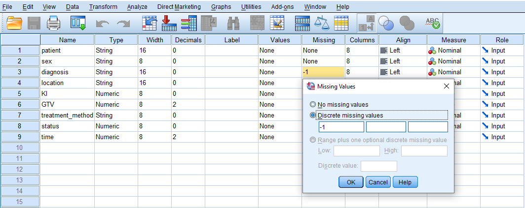
Because our data has missing values shown by the number -1 in some variables, we need to tell SPSS that the -1 values in Diagnosis variable are missing values and not actual values. Therefore, for the Diagnosis variable, we click on Missing and in the window that opens we select Discrete missing values and enter -1 in the first box, as shown in Figure 1.
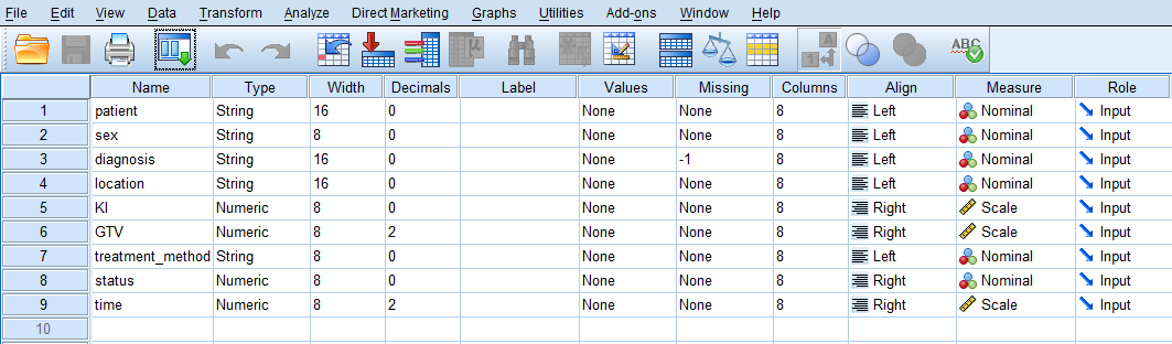
After creating all variables, the Variable View tab of SPSS for our dataset should look like Figure 2.
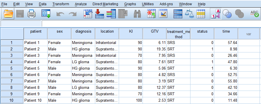
Once the variables are created, we can enter or paste the data into the columns in the Data View tab of SPSS program (the data file can be downloaded from the links above). Figure 3 shows how the data for all variables should look like in the Data View tab (the screenshot shows data for only 10 cases).
We are now ready to conduct Cox regression in SPSS!
Analysis: Cox Regression in SPSS
In a survival analysis, we try to find the probability of survival for a patient after a certain amount of time in a follow-up. In addition, if we are also interested in knowing the effect of an independent variable (a risk factor) on survival probability, we can use a regression method called Cox proportional hazard regression. Similar to regression, Cox regression informs us about the effect of independent variables on the survival probability.
In our example data, we are interested in understanding the relationship between patient sex, tumor location, gross tumor volume, tumor type, patient healthiness index (Karnofsky index), and tumor treatment method with survival probability. We use Cox regression to analyze the data and address this question.
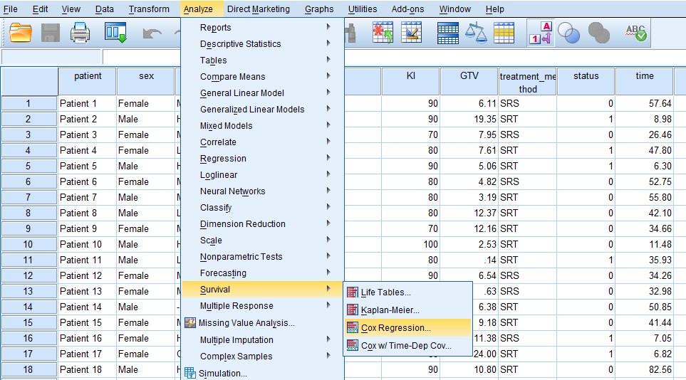
In SPSS, Cox proportional hazard (PH) regression can be accessed through the menu Analyze / Survival / Cox Regression, shown in Figure 4.
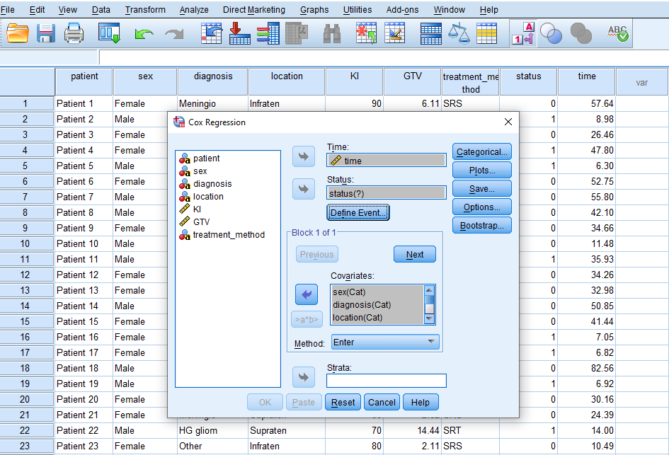
After clicking on Cox Regression, a window will appear asking for Time, Status, and Covariates. We send time into the Time box, Status into the Status box, and the predictor variables (covariates) sex, diagnosis, location, KI, GTV, and treatment method in the Covariate box. (Figure 5.)
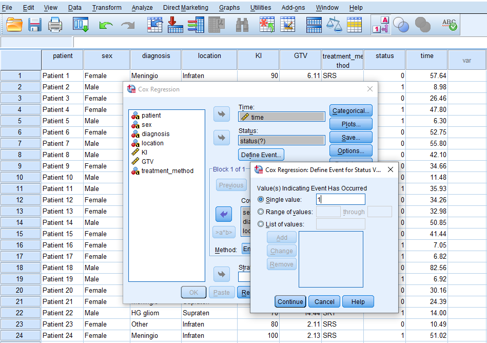
While in this window, we click on Define Event to inform SPSS that the event we are modeling (death of a patient) is denoted by the value 1 in the data. So, we enter 1 in the Single value box (Figure 6) and click on Continue.
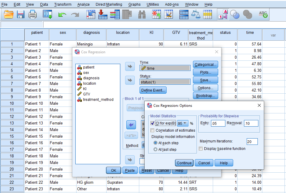
Next, we click on Options and tick CI for exp(B) to obtain confidence interval values for the odds of hazard rate (Figure 7).
We click on Continue and finally on OK to run the Cox proportional hazard regression.
Interpretation: Cox Regression in SPSS
The first table in the SPSS Cox regression output is the Case Processing Summary (Figure 8).
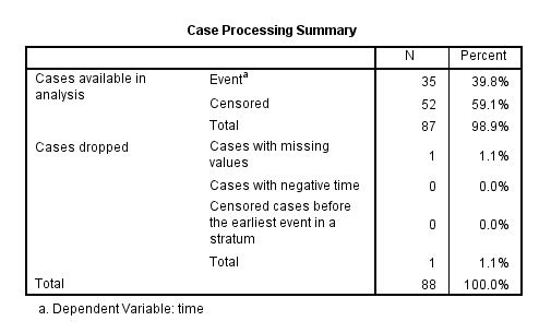
The Case Processing Summary table shows the number of cases processed in the analysis and the number of cases excluded or dropped. The Cases dropped row indicates that 1 case was dropped because we marked it as a missing value. There are 35 cases (39.8%) that experienced the Event (death) and 52 cases (59.1%) that were Censored (survived or were not tracked for non-informative reasons).
The next table in the output is the Categorical Variable Codings (Figure 9).
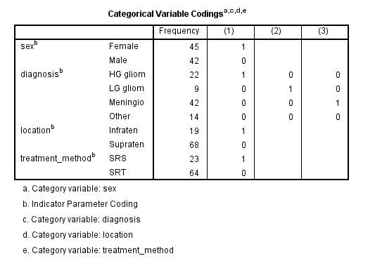
The Categorical Variable Codings table shows only the categorical variables in the data and how their categories (levels) are coded by SPSS in the analysis and the results tables. This method of coding is called dummy coding (or one-hot encoding) where a categorical variable is encoded as many as its categories minus one into binary variables. For example, the categorical variable Diagnosis has four categories, which is in turn encoded as three binary variables where the fourth category is hidden as the reference. In this table we can see that Diagnosis has four categories (HG gliom, LG gliom, Meningio, and Other), but only HG gliom, LG gliom, Meningio receive dummy coding indicated by 1. So, HG gliom is coded as 1 and as the (1) binary variable, LG gliom is coded as 1 as the (2) binary variable, and Meningio is coded as 1 as the (3) binary variable; but the category Other is encoded as 0 in all binary variables, which means that it will not appear in the results and is considered as the reference category (the category all other categories are compared with). The same logic applies to other categorical variables. For example, in categorical variable Sex, Female is encoded as 1 and Male is encoded as 0, which means Male is the reference category (suppressed in the results) and the regression results are shown for Females.
Similar to the logistic regression, SPSS outputs the Cox regression results in blocks because of the nested comparison of statistical metric. Figure 10 shows the results in Block 0 and Block 1.
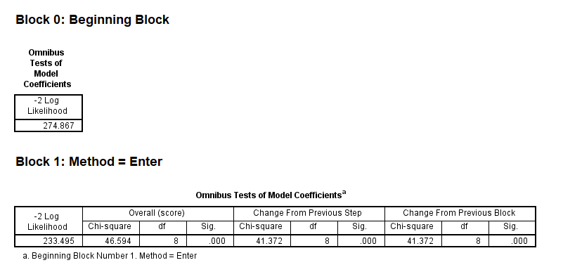
Block 0 shows the -2 Log Likelihood statistic when there are no predictors in the model. We can use this information criterion to compare with the model which has all predictors entered in Block 1. In this way, the effect of adding predictors to the model can be calculated and interpreted. We can see that in Block 0, the statistic is 274.867 and in Block 1 it decreases to 233.495 (the smaller, the better). This decrease is noted in the middle of the table (Change From Previous Step), which is 41.372, and statistically significant. It means that the simultaneous addition of all predictors to the model in Block 0 (null model, then becoming Block 1) has significantly improved model performance (it’s a better model than the null model). So, we conclude that our model is overall significant. But we need to know which predictors have significantly contributed to the model. We can look at the next table to find the effect (coefficients) of the predictors in the model (Figure 11).
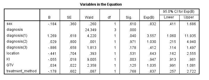
The table of variables and their coefficients in Figure 11 looks like a regression table. The effect of each variable is denoted by the B coefficients (on log-odds scale) and if the effect is significant it is indicated in the Sig column. The column Exp(B) transforms the coefficients from the log-odd scale to odds scale.
According to the coefficients table, the effect of sex is not statistically significant (p = 0.610). Next, the overall effect of the Diagnosis factor is significant (p < 0.05, note that there is no coefficient for the Diagnosis factor, but there are coefficients for each category of the Diagnosis factor, which we will discuss below). The effect of tumor Location is not statistically significant (p = 0.531). The effect of KI is statistically significant (p = 0.003). The effect of GTV is not statistically significant (p = 0.125). Also, the effect of Treatment method is not statistically significant (p = 0.768).
Now, let's interpret the results for statistically significant predictors in the Cox regression. If the B coefficients are negative or if the Exp(B) values are less than 1, the predictor has a decreasing effect on hazard rate. For the KI continuous predictor, for each unit increase in KI, the hazard rate (death) decreases by (1-0.947) x 100 = 5.3% holding all other predictors constant.
For the categorical variable Diagnosis, we can see that there are three coefficients for three out of four categories, indicated by their index numbers diagnosis(1), diagnosis(2), and diagnosis(3). These categories are compared with the fourth category, the reference category. We need to look at the variable encoding table to find out which category is the reference category, and what those index numbers (1, 2, 3) refer to. The categorical encoding table is shown in Figure 9 above, but we show it here again for convenience.
First, let's find out what the reference category is for the Diagnosis factor. The categories in the table are HG gliom, LG glio, Meningio, and Other. Across each category, there are indicator values 1 and 0. The reference category is one whose indicator values are all 0's, which is Other category here. The index number in the Cox regression coefficients table refers to the columns in the table above. For example, diagnosis(1) is the category in column (1) of the Diagnosis factor whose indicator value is 1, which is HG gliom. For category diagnosis(2), we look at column (2) and see which row has indicator 1, which is LG gliom. For category diagnosis(3), we look at column (3) and find the row that has indicator value 1, which is Meningio. Now we go back to the Cox regression coefficients results table, reproduced below.
We can see that only diagnosis(1) has a statistically significant effect (p = 0.040). The hazard rate of HG gliom with respect to Other diagnosis is 3.557 time higher (355.7% higher risk of death) if we hold other predictors constant. The hazard rate of LG gliom (diagnosis 2) is slightly higher than Other diagnosis by only 3% (which is not statistically significant). The hazard rate of diagnosis 3 (Meningio) compared to the reference Other is lower by (1-0.412) x 100 = 58.8% (which is not statistically significant).
Reporting the Results of Survival Analysis
The Cox proportional hazards regression was performed to assess the impact of patients' sex, brain tumor diagnosis, tumor location, Karnofsky Index (KI), gross tumor volume (GTV), and treatment method on survival probability in patients with primary brain tumors. The proportional hazards assumption was verified and met for all covariates. Diagnosis type was modeled with “Other” as the reference category. The effects of sex, tumor location, GTV, and treatment method were not statistically significant (p > 0.05). KI was statistically significant (χ² = 9.005, p < 0.05), with a coefficient of -0.055 and a hazard ratio of 0.947 (95% CI: 0.913-0.981), indicating that higher KI scores were associated with improved survival. Diagnosis type was also statistically significant (χ²=24.349, p < 0.05); patients with HG glioma had a significantly higher hazard ratio (3.557, 95% CI: 1.060-11.936) compared to the “Other” group. Differences between LG glioma and “Other” and between meningioma and “Other” were not statistically significant (p > 0.05).