Survival Analysis in SPSS: Kaplan-Meier Curve
Survival analysis is a collection of statistical methods that model the probability of an event after some time (survival time). In a survival analysis, we are interested to know the probability of an event occurring over a certain period of time and whether the survival probability is different across groups, and similar to regression analysis, what variables or characteristics contribute to the occurrence of that event. The latter inquiry can be addressed by Cox regression. Time-to-event examples may include time to death, failure of a mechanical or electric device, germination of seeds, time it takes for a property to sell, or time it takes for a drug to be effective.

Introduction to Survival Analysis (Kaplan-Meier Method)
In some studies, we are interested in modeling the time it takes for the occurrence of an event. The outcome in these data is the status of an event, such as death from cancer, failure of a mechanical heart valve, wear of vehicle tires, relapse to smoking, or finding a job since graduation day. Such data are collectively called time-to-event data and the statistical methods used to model these data are generally and most commonly called survival analysis. Survival analysis models describe the lifetime of individuals (e.g., cancer patients) or duration of events (e.g., time to failure of a mechanical heart or hip replacement or dental implants). In addition, survival models help us understand if the distribution of survival times is identical across groups, such as female and male patients, treatment methods, or device materials.
The data in a survival analysis has two outcomes: event (cases that experienced the event) and censored (cases that did not experience the event). What makes the survival data different from a binary outcome distribution is the presence of cases which have not experienced the event of interest (e.g., death, failure, relapse) during or after the time frame in which data is collected. For example, in a study on a new drug, the effectiveness of drug is followed up for 12 months. Some patients may drop out and some patients may not show any improvement during the 12-month period. However, we are not sure what happens to those patients who drop out or cannot be followed up after 12 months. As another example, in a study on time-to-germination of seeds, some seeds may be eaten by birds and therefore we do not know their time to germination. Or a property owner may remove their listing from the market, and we do not know how long it would have taken to sell. Such cases are called censored observations and must be included in the analysis.
Survival analysis methods, such as Kaplan-Meier, address this incompleteness (censored observations) in data. Censored observations also include those cases that we know did not experience the event (e.g., did not die, did not break, etc.). The Kaplan-Meier curve is a step function that displays the probability of survival over time, taking into account censored data (e.g., patients who leave the study or are lost to follow-up).
In the following sections, we present an example research scenario where a survival analysis using Kaplan-Meier method will be used to analyze the data. We will demonstrate how to perform survival analysis using Kaplan-Meier method in SPSS step-by-step. In a separate module, we present Cox (proportional hazard) regression to investigate what factors influence survival probability.
Survival Analysis (Kaplan-Meier) Example
What is the survival probability of a patient with primary brain tumor after 24 months of receiving therapy? Is the survival probability equal across male and female patients? Is the survival probability equal across different treatment methods?

A team of doctors and health researchers are interested in understanding the survival probability of primary brain tumor patients receiving treatment with different stereotactic radiation methods at a cancer institute (Masaryk Memorial Cancer Institute Brno). In addition, the researchers are interested in any difference in the effectiveness of the treatment between female and male patients and treatment methods.
For this purpose, the researchers collected data from 88 primary brain tumor patients on their sex (male, female), gross tumor volume (GTV), tumor diagnosis (meningioma, LG glioma, HG glioma, others), the location of the tumor in the brain (infratentorial or supratentorial), Karnofsky index (an index showing health, ranging from excellent health 100% to very poor health 0%), and treatment methods (SRS or SRT). The two treatment methods include SRS (stereotactic radiosurgery) or SRT (stereotactic radiotherapy). The event of interest in this survival analysis was the death of the patients, shown in the status variable (1 = dead, 0 = censored). Time to the event is shown in the time variable (months). Table 1 shows data for five patients in this study.
| Patient | Sex | Diagnosis | Location | Karnofsky Index | GTV | Treatment Method | Status | Time (months) |
|---|---|---|---|---|---|---|---|---|
| Patient01 | Female | Meningioma | Infratentorial | 90 | 6.11 | SRS | 0 | 57.64 |
| Patient02 | Male | HG glioma | Supratentorial | 90 | 19.35 | SRT | 1 | 8.98 |
| Patient03 | Female | Meningioma | Infratentorial | 70 | 7.95 | SRS | 0 | 26.46 |
| Patient04 | Female | LG glioma | Supratentorial | 80 | 7.61 | SRT | 1 | 47.8 |
| Patient05 | Male | HG glioma | Supratentorial | 90 | 5.06 | SRS | 1 | 6.3 |
| ... | ... | ... | ... | ... | ... | ... | ... | ... |
The data for this example can be downloaded in the SPSS format or in CSV format. The data is also available in the supplemental file of the published paper.
Entering Data into SPSS
The data for this example can be downloaded from the links above. If you have downloaded the SPSS format of the data, double-click on the file to open the file. Alternatively, you can open the file through SPSS menu bar using the File / Open / Data. If the downloaded file is in the CSV format, in SPSS you can use File / Read text data to open a step-by-step window (wizard) to open the CSV file.
To enter the data in the SPSS program manually (entering data by hand or pasting the data into SPSS from a spreadsheet), first we click on the Variable View tab (bottom left) and create the variables under name column: patient, sex, diagnosis, location, KI, GTV, treatment method, status, and time.
When defining the variables, specify both the data type and the measurement level for SPSS. The data type is used by the SPSS software to understand the data type (e.g., text, numbers, dates, etc.), while the measurement level helps the statistical algorithm for running the appropriate analysis. We specify the following attributes for each variable:
- patient: Type is string. Width is 16. Measure is Nominal.
- sex: Type is string. Width is 8. Measure is Nominal.
- diagnosis: Type is string. Width is 8. Measure is Nominal. Missing = -1
- location: Type is string. Width is 8. Measure is Nominal.
- KI: Type is Numeric. Measure is Scale.
- GTV: Type is Numeric. Measure is Scale.
- treatment_method: Type is string. Width is 8. Measure is Nominal.
- status: Type is Numeric. Width is 8. Measure is Nominal.
- time: Type is Numeric. Measure is Scale.
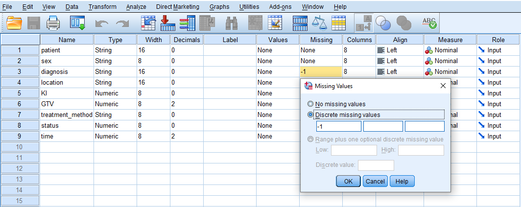
Because our data has missing values shown by the number -1 in some variables, we need to tell SPSS that the -1 values in Diagnosis variable are missing values and not actual values. Therefore, for the Diagnosis variable, we click on Missing and in the window that opens we select Discrete missing values and enter -1 in the first box, as shown in Figure 1.
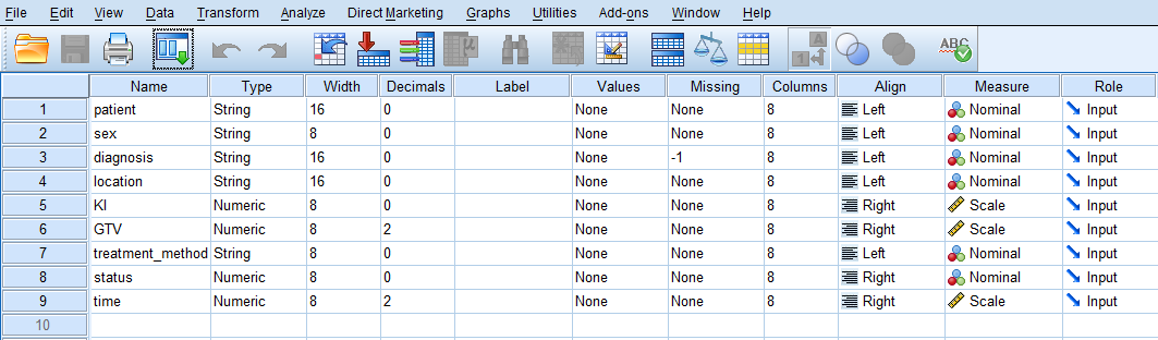
After creating all variables, the Variable View tab of SPSS for our dataset should look like Figure 2.
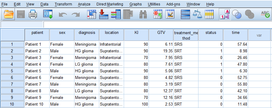
Once the variables are created, we can enter / paste the data into the columns in the Data View tab of SPSS program (the data file can be downloaded from the links above). Figure 3 shows how the data for all variables should look like in the Data View tab (the screenshot shows data for only 10 cases).
We are now ready to conduct survival analysis using Kaplan-Meier method in SPSS!
Analysis: Survival Analysis (Kaplan-Meier) in SPSS
In a survival analysis, we try to find the probability of survival for a patient after a certain amount of time in a follow-up. In addition, if there is a grouping variable in the data, such as sex, treatment method, or dosage, survival analysis can also address the question if such a survival probability is different across the groups. These questions can be addressed using the Kaplan-Meier method (for producing the survival probability curve over time period) and the log-rank test (for testing group difference). If we are also interested in knowing the effect of an independent variable (risk factor) on the survival probability, we can use a regression method called Cox proportional hazard regression. Similar to regression, Cox regression informs us about the effect of an independent variable on the survival probability.
In our example data, we are interested in obtaining survival probability curve (also know as Kaplan-Meier curve) and investigating if the survival probability is different across sex (using log-rank test).
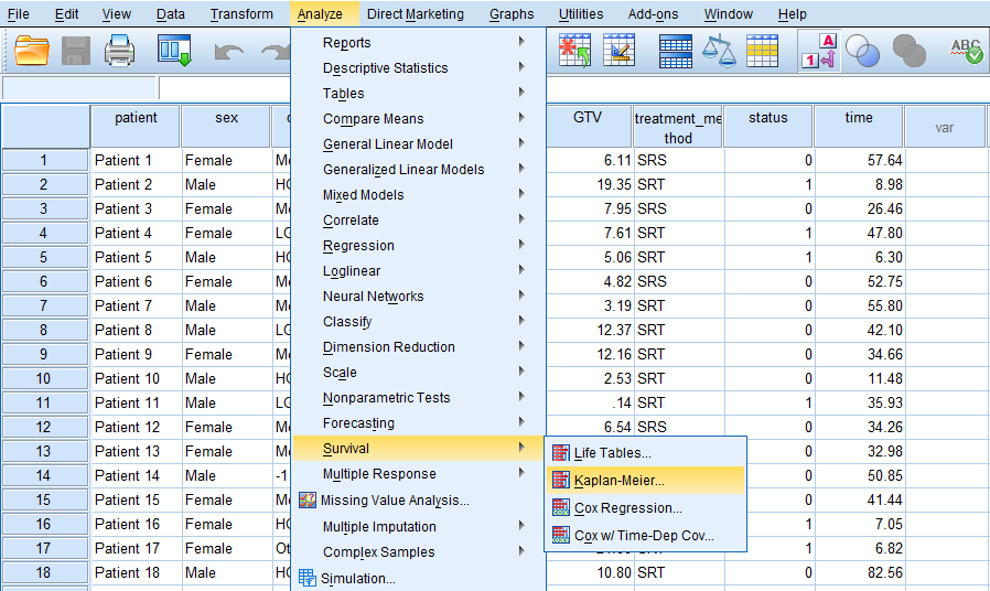
In SPSS, survival analysis using Kaplan-Meier method can be accessed through the menu Analyze / Survival / Kaplan-Meier, as shown in Figure 4.
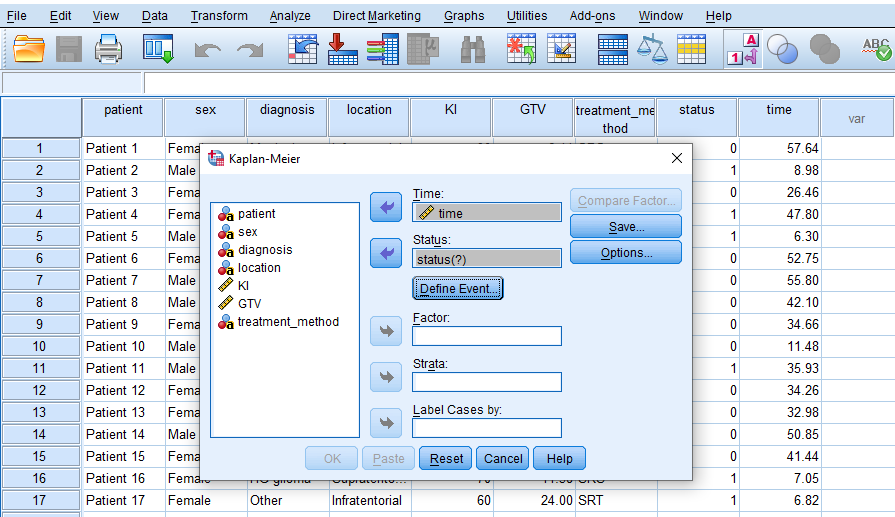
After clicking on Kaplan-Meier, a window will appear asking for Time and Status (event). We send time into the Time box and Status into the Status box (Figure 5.)
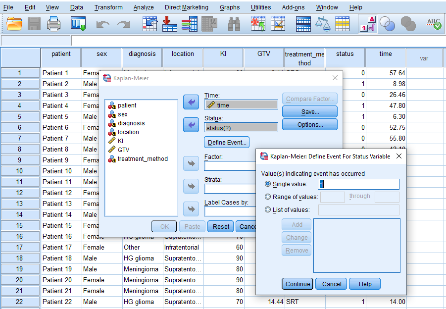
While in this window, we click on Define Event to inform that the event we are modeling (death of a patient) is denoted by the number 1 in the data. So, we enter 1 in the Single value box (Figure 6) and click on Continue.
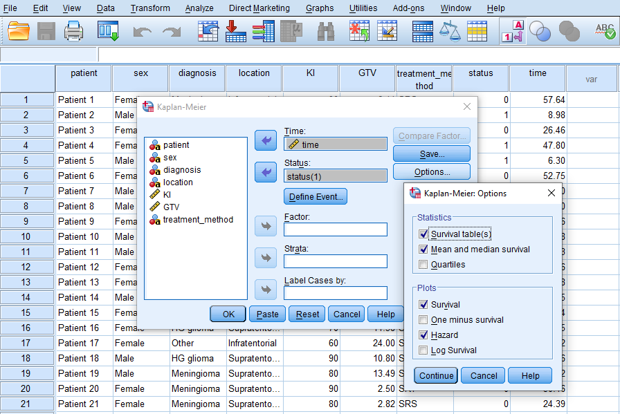
Next, we click on Options and tick Survival tables, Mean and median survival, and in the Plots section we tick Survival and Hazard (Figure 7).
We click on Continue and finally on OK to run the survival analysis for all patients (ignoring any grouping factor).
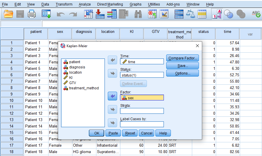
Another question that we would like to address here is if the survival probability is different across sex and if the difference is statistically significant. We run the analysis again following the steps above except that we add sex as factor (Figure 8).
Because we want to compare female and male patients, we click on Compare Factor and choose the log-rank test (Figure 9).
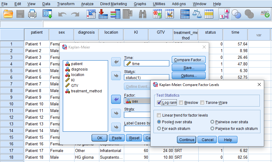
We click on Continue and finally click on OK.
Interpretation: Survival Analysis (Kaplan-Meier) in SPSS
Part I: All Patients
The first table in the SPSS output from the Kaplan-Meier analysis is called Case Processing Summary (Figure 10).
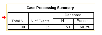
According to this table, there are 88 patients in the data set. The number of events records the number of deaths (Status = 1), so out of 88 patients, 35 died at different times of the treatment period. Censored includes patients who survived or who left the treatment program, or who we do not have any information about what happened to them (dead or alive) once the treatment was ended. There are 53 censored patients (60.2%).
The next table in the SPSS output is called the Survival Table (Figure 11).
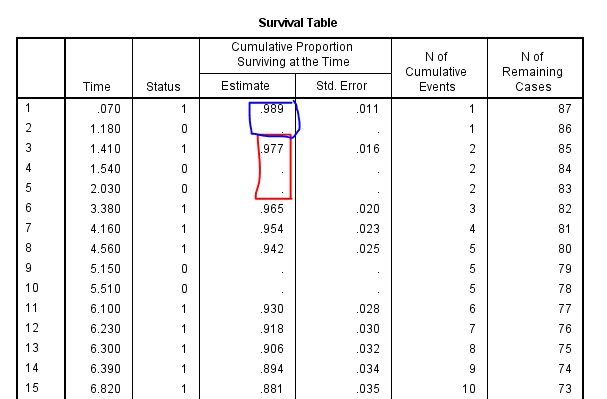
The Survival Table lists all patients in the data (here we have included only 15 patients), their Time to event (months), their Status (1 = died, 0 = censored), Cumulative Proportion Surviving at the Time (survival probability), Number of Cumulative Events (how many patients died until this time), and Number of Remaining Cases. The data is sorted in ascending order by Time. Patient 1 had an event (death) at time 0.070 (month). This patient's status is recorded as 1, meaning this patient died. Based on this information (death at time 0.07), the probability of survival (not dying) estimated based on Kaplan-Meier method is 0.989 (with standard error = 0.011). In the column N of Cumulative Events, the number is 1, because until this time 1 patient had died and the remaining (87) had survived. Next, Patient 2 had a Status = 0 at time 1.180, meaning that this person was censored (no longer in the treatment program, neither died). Because at this time no event occurred, the survival probability remains unchanged. SPSS shows unchanged survival probability with a dot, which means that the value should be read from the prior immediate probability (0.989). Because this person is censored (out of program), the number of remaining cases decreases to 86.
The descriptive statistics for our data set are displayed in the next table in the output, Means and Medians of Survival Time (Figure 12).
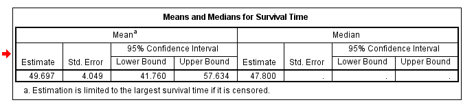
The mean survival time is 49.697 months, and the median survival time is 47.800 months. In survival analysis, the median survival time is typically reported because of the skewed nature of the data distribution.
Finally, we get two plots. The first plot shows the survival probability over time for all patients (Figure 13).
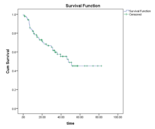
In Figure 13, the survival probability is shown on the Y (vertical) axis and time is shown on the X (horizontal axis). If we know how long a patient has been in the treatment plan, we can estimate their survival probability. For example, for a patient in the treatment plan for 40 months, their survival probability is about 0.55 (which can also be read from the Survival Table). The plus signs on the curve indicate censored cases.
The second plot shows the hazard function (Figure 14).
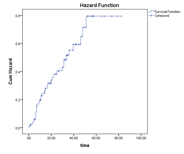
Hazard is the opposite of survival. The hazard function plot shows the probability of death at a certain time. As Figure 14 shows, the probability of death increases as we approach the end of the program.
Part II: Comparing Survival Probability for Female and Male Patients
When we added sex as a factor, SPSS runs the Kaplan-Meier analysis separately for female and male patients and also produces the results of the log-rank test. So, we see in the output, similar to the tables to single-group analysis, Case Processing Summary and Means and Medians for Survival Time are produced for female and male patients (Figures 15 and 16).
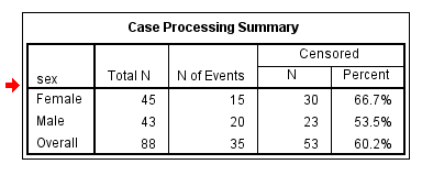
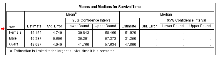
The median survival time among female patients is 51.020 months while that of male patients is 31.250 months. Is the difference statistically significant? We look at the results of the log-rank test in Figure 17.
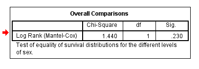
The log-rank test (also called Mantel-Haenszel test) is based on the chi-square statistic and distribution. According to the log-rank test, there is not a statistically significant difference between female and male patients in terms of survival probability (chi-square = 1.440, df = 1, p = 0.230). Figures 18 and 19 show the survival and hazard plots for female and male patients.
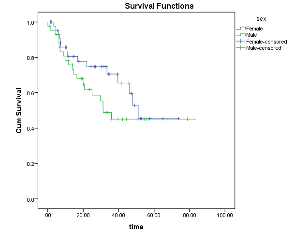
In Figure 18 we can see that at some time intervals male patients have lower survival probability than female patients. However, the difference becomes negligible or none after about 51 months.
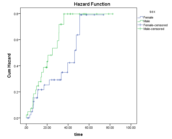
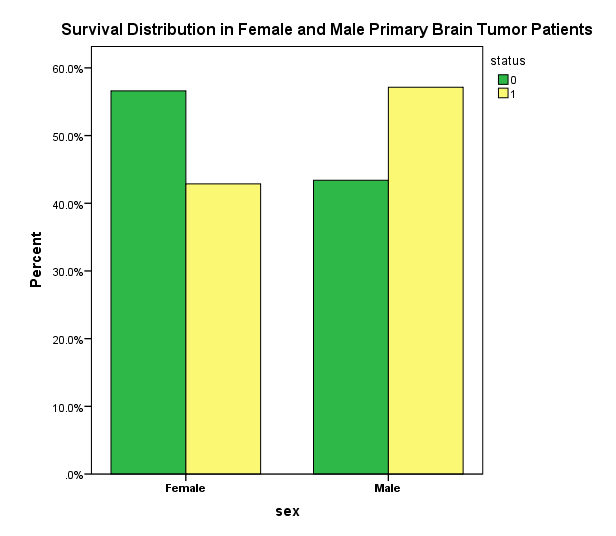
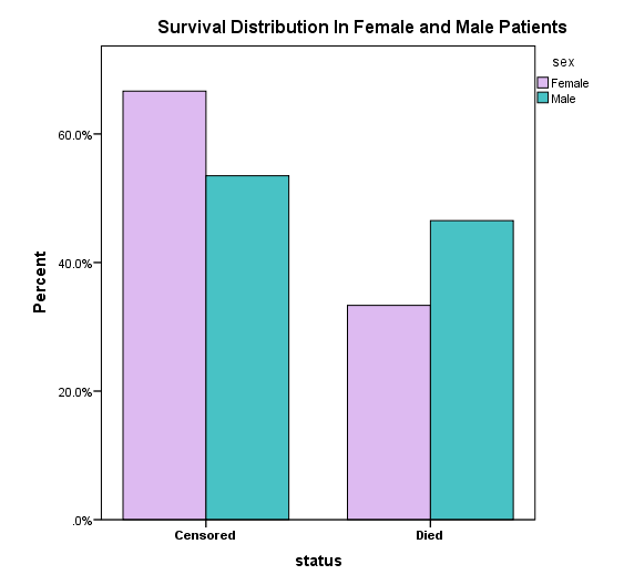
Similarly, the hazard function plot in Figure 19 shows that the hazard difference between female and male patients becomes negligible from month 51. Figures 20 and 21 show the survival distribution in female and male patients.
If we want to know whether the survival probability is different between treatment methods, we can run the analysis again but use treatment method instead of sex as factor (replace sex with treatment method, as shown in Figure 8). When comparing survival probability between groups, the effect of cohort characterstics, such as patient age, should also be considered as potential confounders.
Reporting the Results of Survival Analysis
A Kaplan-Meier survival analysis was conducted to compare survival distributions across female and male primary brain tumor patients. Median survival times for female and male patients were 51.02 and 31.2 months, respectively. The log-rank test indicated a non-significant difference in survival distributions, χ²(2) = 1.44, p = 0.23.